JPEG quality estimation using simple least squares matching of quantization tables
In my previous post I addressed several problems I ran into when I tried to estimate the “last saved” quality level of JPEG images. It described some experiments based on ImageMagick’s quality heuristic, which led to a Python implementation of a modified version of the heuristic that improves the behaviour for images with a quality of 50% or less.
I still wasn’t entirely happy with this solution. This was partially because ImageMagick’s heuristic uses aggregated coefficients of the image’s quantization tables, which makes it potentially vulnerable to collisions. Another concern was, that the reasoning behind certain details of ImageMagick’s heuristic seems rather opaque (at least to me!).
In this post I explore a different approach to JPEG quality estimation, which is based on a straightforward comparison with “standard” JPEG quantization tables using least squares matching. I also propose a measure that characterizes how similar an image’s quantization tables are to its closest “standard” tables. This could be useful as a measure of confidence in the quality estimate. I present some tests where I compare the results of the least squares matching method with those of the ImageMagick heuristics. I also discuss the results of a simple sensitivity analysis.
JPEG quality and standard quantization tables
ImageMagick’s JPEG quality heuristic is based on the “standard” quantization tables that are defined in Annex K of the JPEG standard. Its overall objective seems to be to match an image’s quantization tables with the most similar “standard” quantization tables. Since the quality level of each of these “standard” tables is known, this then provides the quality estimate.
ImageMagick’s heuristic does this in an indirect (and to me somewhat opaque) way, possibly to avoid computational cost. This post explores a more straightforward approach, which simply compares the coefficients in an image’s quantization tables against the corresponding coefficients in the “standard” tables, and then returns the quality level of the best match1.
Scaling of standard tables to quality levels
To understand how this works, it’s first important to know that Annex K in the JPEG standard describes two “standard” “quantization tables for luminance and chrominance. Here’s the luminance table:
| 16 | 11 | 10 | 16 | 24 | 40 | 51 | 61 |
| 12 | 12 | 14 | 19 | 26 | 58 | 60 | 55 |
| 14 | 13 | 16 | 24 | 40 | 57 | 69 | 56 |
| 14 | 17 | 22 | 29 | 51 | 87 | 80 | 62 |
| 18 | 22 | 37 | 56 | 68 | 109 | 103 | 77 |
| 24 | 35 | 55 | 64 | 81 | 104 | 113 | 92 |
| 49 | 64 | 78 | 87 | 103 | 121 | 120 | 101 |
| 72 | 92 | 95 | 98 | 112 | 100 | 103 | 99 |
This is the base table with coefficients that are valid for quality level 50. The tables for all other quality levels can be derived from this base table using Equations 1 and 2 from this paper by Kornblum (2008)2. First, for each quality level Q we can calculate a corresponding scaling factor S:
S is then used to calculate scaled quantization coefficients Tis from the base coefficients Tib using the following equation:
Here i is the ith element in the table. Note the floor brackets, which mean the expression inside them is rounded down to the nearest integer number. For 8-bit quantization tables (which is the most common situation) the scaled coefficients also need to be capped at a maximum of 255.
As an example, applying these equations to Q=75 results in a scaling factor S of 15000, and the quantization coefficients become:
| 8 | 6 | 5 | 8 | 12 | 20 | 26 | 31 |
| 6 | 6 | 7 | 10 | 13 | 29 | 30 | 28 |
| 7 | 7 | 8 | 12 | 20 | 29 | 35 | 28 |
| 7 | 9 | 11 | 15 | 26 | 44 | 40 | 31 |
| 9 | 11 | 19 | 28 | 34 | 55 | 52 | 39 |
| 12 | 18 | 28 | 32 | 41 | 52 | 57 | 46 |
| 25 | 32 | 39 | 44 | 52 | 61 | 60 | 51 |
| 36 | 46 | 48 | 49 | 56 | 50 | 52 | 50 |
This way it is possible to calculate the quantization tables for all 100 quality levels. For the chrominance tables the same procedure can be used.
Estimating quality from scaled tables
For a given JPEG file, the quality can then be estimated by comparing its quantization tables against each of the scaled tables that are derived from the standard tables. As a basis for this comparison we can calculate, for each quality level, the sum of squared errors between the coefficients in the image’s quantization table and the corresponding coefficients in the scaled standard table. For an image with 2 quantization tables (one for luminance and another one for chrominance) this is given by:
Here, Tilum and Tichrom represent the coefficients for luminance and chrominance from the image’s quantization table, and Tis,lum and Tis, chrom are the corresponding coefficients from the (scaled) standard tables.
Repeating this for all quality levels results in 100 SSE values. The quality level with the smallest SSE value is then our best estimate for the quality of the image. An SSE value of exactly 0 means the image uses the standard JPEG quantization tables. In that case we can be confident that our estimate is the exact quality level at which the image was compressed. Larger values indicate the use of non-standard quantization tables, in which case the quality estimate may be less accurate.
Characterizing similarity to standard tables
For images that don’t use the standard quantization tables, it would be useful to have some measure that expresses how much the quantization tables deviate from the best matching standard table. This could be used as a measure of confidence in the quality estimate. By itself, SSE is not a good measure of this. Firstly, it is influenced by the number of quantization tables in the image. We could remove this influence by transforming the SSE value to a root mean squared error (RMSE):
Here, tables is the number of quantization tables (which is either 1 or 2). The interpretation of these RMSE values is still complicated by the fact that the quantization coefficients are significantly larger at lower quality levels. In practice this has the effect that the RMSE values are generally much larger at low quality levels relative to higher quality levels, even for images with a similar overall “fit” to a standard quantization table.
One “goodness of fit” measure that does not have this drawback is the Nash–Sutcliffe efficiency coefficient (NSE). It is mostly used in the field of hydrology to characterize how well the output of hydrological simulation models agrees with observations. Here, we will use it to characterize how well the coefficients in the standard table agree with those in the image’s quantization table. Rewritten for our quantization coefficients, NSE is given by:
Here Ti represents the ith coefficient from the image’s quantization tables, and Tis is the corresponding coefficient from the (scaled) standard tables. N is the total number of coefficients in the image’s quantization tables. Note that, unlike in the SSE equation, the luminance and chrominance coefficients are lumped here for simplicity. Finally, T is the mean of all coefficients Ti in the image’s quantization tables. The interpretation of NSE is quite straightforward:
- A value of 1 indicates a perfect agreement between the image quantization tables and the corresponding standard tables.
- For a value of 0, the standard tables are as good (or rather, bad) an approximation of the image’s quantization tables as T.
- Negative values indicate an extremely poor agreement.
As an example, the below scatter plot shows the quantization coefficients (T) from one of out dbnl master images, plotted against the corresponding coefficients (Ts) from the best matching standard table. It also shows the line of perfect agreement (green, dashed), the quality estimate, the root mean squared error, and the Nash-Sutcliffe Efficiency:
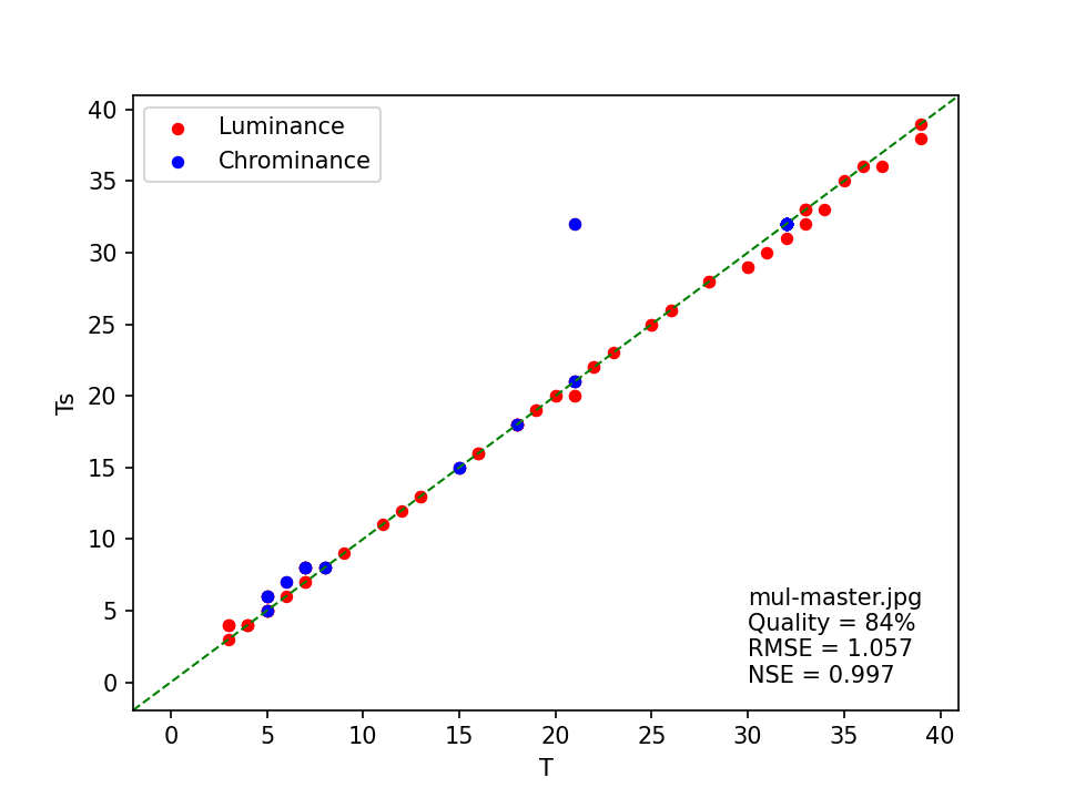
The plot shows that, aside from one outlier in the chrominance table, the image’s quantization coefficients are closely approximated by those in the standard quantization tables. This is reflected by the NSE value, which is close to 1. Now compare this with the plot I made for the corresponding access image:
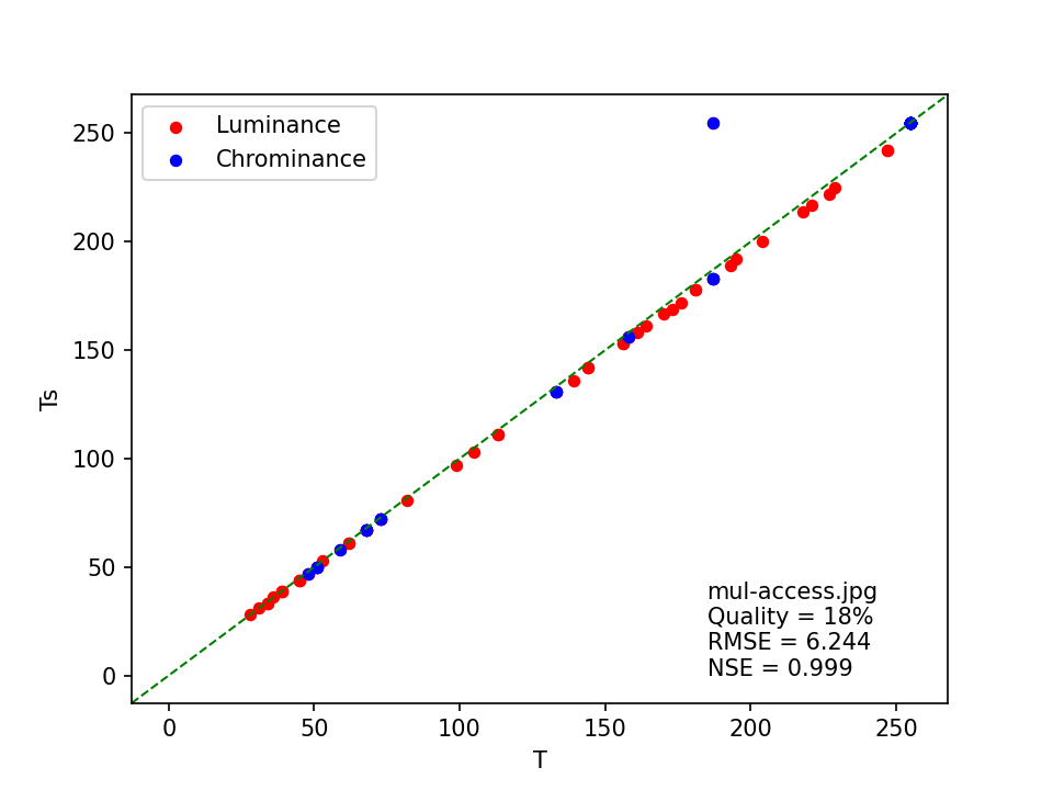
Visually, the agreement between the standard quantization table coefficients and those of the image looks very similar to the previous plot. But note how the RMSE value is much larger here, which is caused by the much larger overall coefficients in the quantization tables. However, this doesn’t have any effect on NSE, which is even marginally closer to 1 than for the master image.
By contrast, things are very different for this image:

The plot shows that the standard JPEG tables are a relatively poor approximation here, and this is refected by the low NSE value. A similar case is this image:
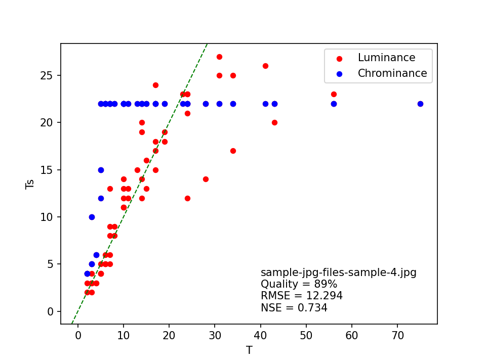
Despite the different quality estimate and RMSE value, this visually looks like it’s in the same ballpark as the previous image, and the similar NSE value confirms this.
Based on these examples, NSE appears to give a good indication of the fit between the image and standard quantization coefficients. This makes it useful as a measure to asses the confidence in the method’s quality estimates.
Python implementation of least squares matching method
I created a test script with a Python implementation of the method. Apart from the quality estimate, it also reports the corresponding RMSE and NSE values.
Tests with Pillow and ImageMagick JPEGs
As a first test I ran the script on the Pillow and ImageMagick JPEGs I discussed in my previous post. This gave the following result:
| Qenc | Qest(PIL) | RMSE(PIL) | NSE(PIL) | Qest(IM) | RMSE(IM) | NSE(IM) |
|---|---|---|---|---|---|---|
| 5 | 5 | 0.0 | 1.0 | 5 | 0.0 | 1.0 |
| 10 | 10 | 0.0 | 1.0 | 10 | 0.0 | 1.0 |
| 25 | 25 | 0.0 | 1.0 | 25 | 0.0 | 1.0 |
| 50 | 50 | 0.0 | 1.0 | 50 | 0.0 | 1.0 |
| 75 | 75 | 0.0 | 1.0 | 75 | 0.0 | 1.0 |
| 100 | 100 | 0.0 | 1.0 | 100 | 0.0 | 1.0 |
Here Qenc is the encoding quality, and Qest(PIL) and Qest(IM) are the script’s estimates for the Pillow and ImageMagick images, respectively. The script correctly reproduced the encoding quality for all test images. The values RMSE=0 and NSE=1 also indicate that all images use the standard JPEG quantization tables.
Comparison of quality estimation methods
Far more interesting is the behaviour for images that don’t use the standard tables. The previous section already showed the results for the dbnl master and access JPEGs that started this work. To test the method on a more diverse selection of images, I downloaded JPEGs from a variety of sources3. I then ran them through this test script that estimates the JPEG quality using my Python port of the original ImageMagick heuristic, the modified ImageMagick heuristic from my previous post, and the least squares matching method. I then identified images for which one or more of these methods came up with different results, and added a selection of them to this dataset. The following table shows the results of the script for this dataset:
| File | Q (im) |
Q (im, mod) |
Exact (im, mod) |
Q (lsm) |
RMSE (lsm) |
NSE (lsm) |
|---|---|---|---|---|---|---|
| psgradient.jpg | 92 | 92 | False | 93 | 4.438 | 0.747 |
| hopper_16bit_qtables.jpg | na | 1 | False | 13 | 0.795 | 1.0 |
| image-177.jpg | 63 | 63 | True | 81 | 20.509 | 0.732 |
| image-98.jpg | 63 | 63 | True | 81 | 20.509 | 0.732 |
| jpeg420exif.jpg | 90 | 90 | False | 89 | 0.424 | 0.999 |
| jpeg422jfif.jpg | 96 | 96 | False | 97 | 0.0 | 1.0 |
| jpeg444.jpg | 60 | 60 | False | 75 | 0.0 | 1.0 |
| sample-birch-400x300.jpg | 95 | 95 | False | 94 | 3.188 | 0.838 |
| sample-jpg-files-sample-4.jpg | 78 | 78 | True | 89 | 12.294 | 0.734 |
| tapedeck1.jpg | 90 | 90 | False | 93 | 0.753 | 0.992 |
| tapedeck2.jpg | 92 | 92 | False | 95 | 0.421 | 0.996 |
Here Q(im) is the quality estimate from the original ImageMagick heuristic, Q(im), mod is the quality estimate from the modified ImageMagick heuristic, Q(lsm) is the quality estimate from the least squares matching method. In addition Exact(im, mod) is the “exactness” indicator of the modified ImageMagick heuristic, and RMSE(lsm) and NSE(lsm) are the root mean squared error and Nash-Sutcliffe Efficiency values reported by the least squares matching method, respectively.
Below I highlight some of the more interesting results.
jpeg444.jpg
For this image, both the original and modified ImageMagick heuristics estimate the quality at 60%, with no “exact” match. By contrast, the least squares matching method came up with a quality of 75%, with RMSE and NSE indicating a perfect match with the standard JPEG quantization tables. This is comfirmed by plotting the coefficients from the quantization tables against the standard coefficients:
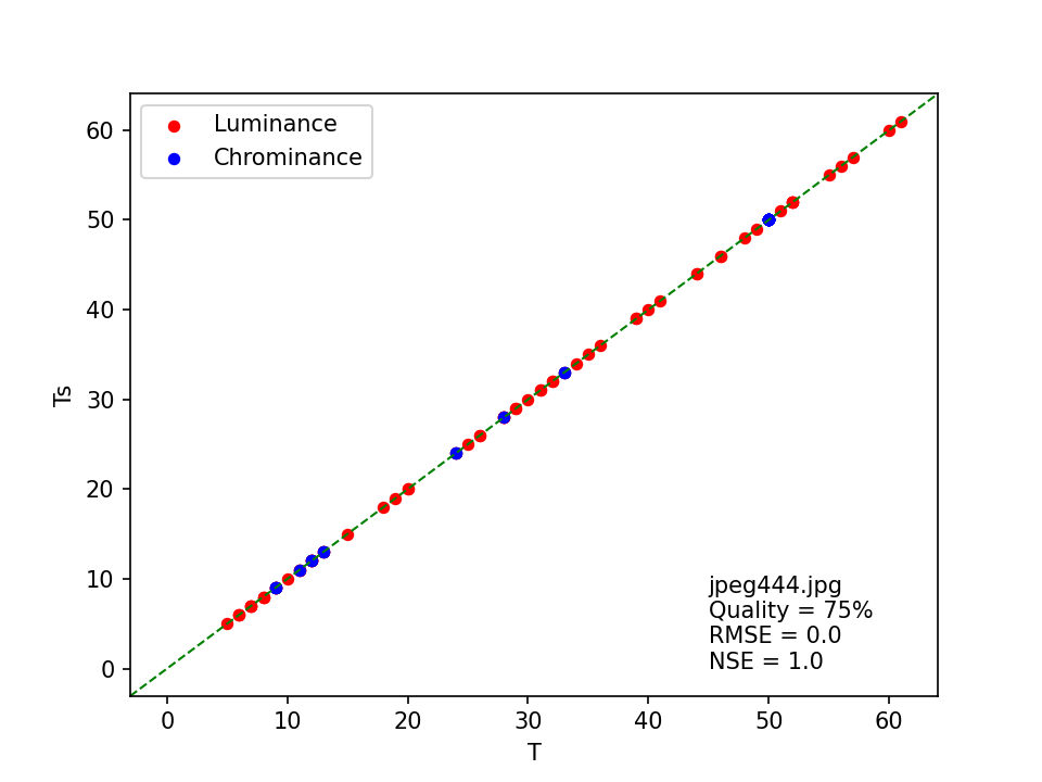
I double-checked the result by uploading the image to FotoForensics, which also came up with 75% quality, and an exact match with the standard tables.
image-98.jpg
Here, the quality is estimated at 63% by both the original and modified ImageMagick heuristics, with an “exact” match. However, the least squares matching method results in a much higher (81%) quality, but the relatively low NSE value of 0.732 indicates a poor fit to the standard JPEG tables. This is confirmed by the scatter plot of T against Ts :
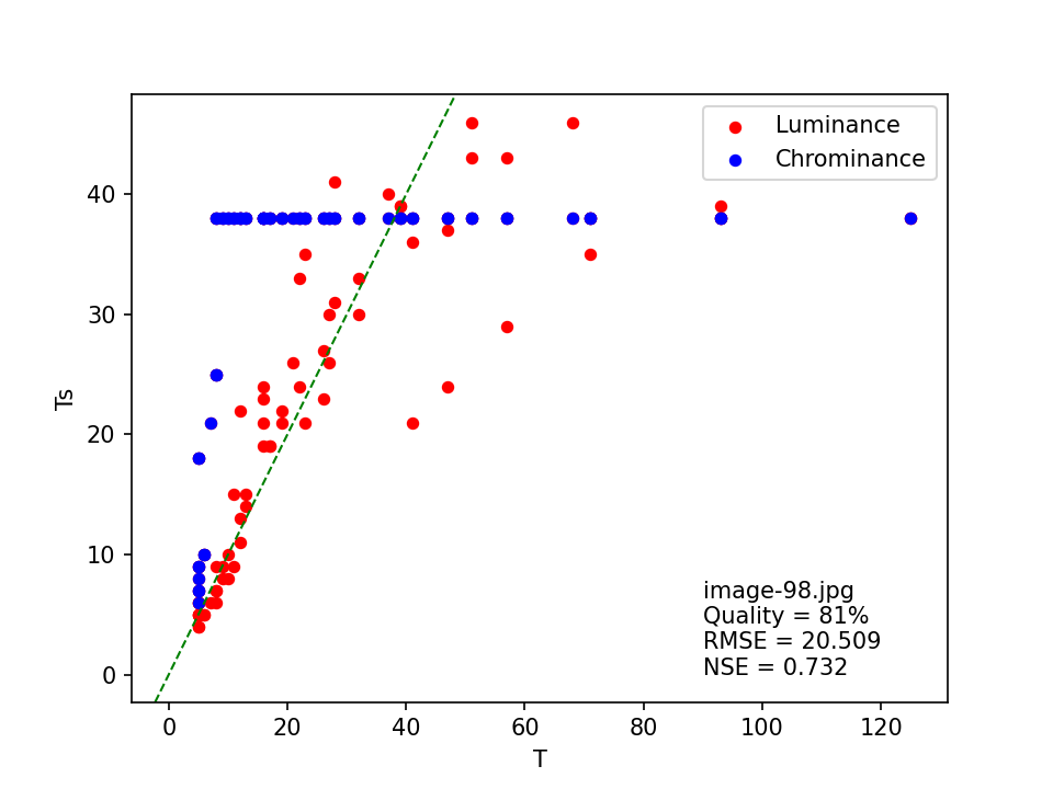
The FotoForensics result also indicates a quality of 81%.
hopper_16bit_qtables.jpg
This image is interesting for a number of reasons. ImageMagick’s original heuristic fails to come up with a quality estimate, while the modified ImageMagick heuristic returns a 1% estimate. Meanwhile, the least squares matching method estimates the quality at 13%. Here’s the corresponding scatter plot:
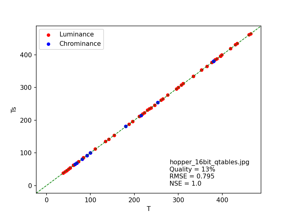
The coefficients in the JPEG quantization tables are usually stored as 8-bit unsigned integers, which means the highest possible value is 255. This particular image uses 16-bit values instead, which we can see from the range of T values in the plot, which goes all the way up to 380! ImageMagick’s heuristic is unable to deal with this4, which results (for the modified version) in an unrealistically low value. The least squares matching method explicitly checks for coefficients outside the 8-bit range, and adjusts its calculations accordingly. Its quality estimate corresponds to the assessment by FotoForensics.
One detail that caught my attention is the non-zero RMSE value, which at first sight seems at odds with the reported NSE value of 1.0. On closer inspection, it turned out that NSE is actually marginally smaller than 1 here, but this is obscured by rounding the reported values at 3 decimals5.
sample-jpg-files-sample-4.jpg
Both ImageMagick heuristics estimate the quality of this image at 78% with an “exact” match, whereas the least squares matching method gives a much higher estimate of 89% (with quite a poor fit with the standard tables). The corresponding FotoForensics estimate is marginally different from this at 88%, but still very close. For completeness here’s its scatter plot (again):

Conclusions from this comparison
Even though the tests presented here are quite limited, the differences that can occur between the quality estimates by the least squares matching method and the ImageMagick heuristics are quite striking. What surprised me in particular, was that even for JPEGs that use the standard quantization tables, ImageMagick’s heuristic may still provide quality estimates that are quite inaccurate. Of course, a major limitation here is the lack of reliable “ground truth” in the form of known quality settings at the time the test images were created. However, the good agreement between the quality estimates of the least squares matching method and the FotoForensics service does inspire some confidence in the methodology.
Another surprise was that ImageMagick’s “exactness” flag isn’t actually indicative of an exact match with the standard JPEG tables. None of the test images for which it returned a “True” value actually contains standard quantization tables, whereas the two images that do contain standard tables resulted in a “False” value!
Sensitivity analysis
To get a better impression of how the method behaves with non-standard quantization tables, I did a simple sensitivity analysis using the cjpeg utility that is part of libjpeg. This tool supports compression with separate quality levels for the luminance and chrominance tables. I used this to compress one source image to all possible quality level combinations. This resulted in 10,000 images, which I then ran through the least squares matching method.
The plot below shows the distribution of estimated quality values Qlsm against Qav, which are the corresponding averages of encoding qualities Qlum and Qchrom6:
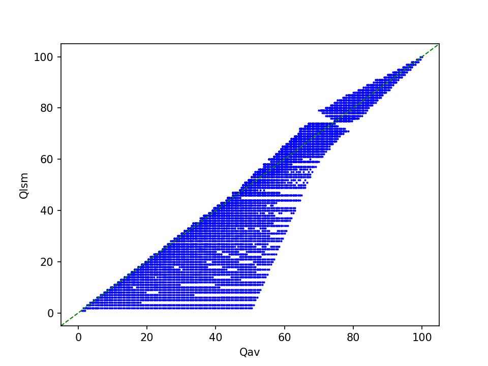
At low average encoding qualities, the bandwidth of corresponding estimates by the least squares matching method is very wide, but this narrows considerably towards higher quality levels.
Another, probably more useful view on the results appears if we plot the quality estimation errors, here expressed as absolute differences between Qav and Qlsm, against the Nash-Sutcliffe Efficiency coefficients:
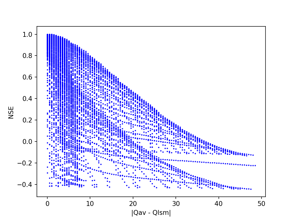
This shows a strong association between NSE values in the upper range with small prediction errors. At lower NSE values, the range of prediction errors becomes progressively wider. Thus, this demonstrates how NSE can be useful as a measure of confidence in the quality estimate.
Performance
One potential concern about the least squares matching method might be that it is computationally not very efficient: for each image, the analysis typically involves 200 comparisons of 64-element tables. Out of interest I did a little performance test using this collection of 700 JPEGs. I analyzed these files with my scripts with the Python ports of the original and modified ImageMagick heuristics, and the least squares matching method.
For each script run, I first ran this command to empty the cache memory:
sudo sysctl vm.drop_caches=3
I then ran each script like this:
(time python3 ./jpeg-quality-demo/jpegquality-lsm.py ./sample-images/images/*.jpg > sample-images.txt) 2> time-lsm.txt
The “time” command results in 3 performance metrics, The most important of which are:
- “real” - the actual amount of time passed between starting the script and its termination.
- “user” - actual CPU time used in executing the process7.
Below table shows these metrics for the three scripts8:
| Method | time (real) | time (user) |
|---|---|---|
| im original | 0m7,624s | 0m3,321s |
| im modified | 0m7,215s | 0m2,968s |
| lsm | 0m13,134s | 0m8,673s |
This shows the least squares matching method is almost 3 times slower than the ImageMagick heuristics in terms of “user” time, and about 2 times slower in terms of “real” time. This translates to an average processing time of 0.01 to 0.02 s per file. Therefore, the reduced performance shouldn’t be any problem in practical terms.
Final thoughts
I originally wrote the least squares matching method code in an attempt to better understand JPEG quality estimation, and to make a more informed assesment of how ImageMagick’s heuristic works. Based on the tests described here, I think I ended up with something that might actually be quite useful, and preferrable to either the original or modified ImageMagick heuristic.
By itself the method isn’t in any way novel, as it’s basically just another implementation of the “Approximate Quantization Tables” quality estimation method as described by Neal Krawetz9. I expect many other, very similar implementations exist that I’m simply not aware of, particularly in the digital forensics domain. This makes it all the more surprising that these apparently haven’t made it to popular image processing and analysis software like ImageMagick. The use of the Nash-Sutcliffe Efficiency as a measure of confidence in the quality estimate may be somewhat novel, but I wouldn’t be surprised if other (and possibly better) methods for this exist.
Finally, it’s important to be aware that the characterization of JPEG quality using the 1 - 100 scale that follows from the “standard” quantization tables is by itself pretty arbitrary10. Essentially, the corresponding “quality” values are just pointers to sets of quantization tables that only have ordinal significance (i.e. higher values mean better quality), but not much more. Due to its wide use, and the lack of any better alternative, it’s still a useful benchmark. This is also why I think it’s important to provide some information on the similarity of an image’s quantization tables to the “standard” ones, as this helps assessing the confidence in the quality estimate.
As always, any feedback and suggestions in response to this post are very welcome!
Scripts and test data
- jpeg-quality-demo Github repository - Github repo with all scripts and test data that were used in this analysis.
- jpegquality-lsm.py - Python implementation of the least squares matching method.
Important note on Python Pillow version
The Python implementation of the least squares matching method (and most of the other scripts as well) requires a recent version of the Pillow Imaging Library. This is because around the release of version 8.3 (I think) Pillow changed the order in which it returns the values inside JPEG quantization tables (details here). All scripts in the repo expect the current/new behaviour, and they will give very wrong results when used with older Pillow versions!
Revision history
- 1 November 2024: added paragraph on significance of JPEG quality scale; added sensitivity analysis.
-
This corresponds to the “Approximate Quantization Tables” method that is mentioned on (and used by) Neal Krawetz’s FotoForensics site (but the site doesn’t provide any details about the implementation). ↩
-
See also this post on StackOverflow. ↩
-
Most notably sample-images, samplelib.com, toolsfairy.com, w3.org and the Pillow source repository. ↩
-
This is because its hard-coded
sumsandhasheslists (see my previous post) are based on 8-bit values. ↩ -
In this case the numerator of the NSE equation (the SSE value) was 81, and the denominator (the variance of the quantization coefficients) 7743557. This results in NSE = 1 - (81/7743557) = 0.99998954, which is reported as 1.0 when rounded to 3 decimals. Meanwhile RMSE = √(81/128) = 0.795. ↩
-
The actual significance of Qav is somewhat questionable, especially for extreme high/low combinations of Qlum and Qchrom. ↩
-
For a more in-depth explanation of these metrics see: https://stackoverflow.com/a/556411/1209004 ↩
-
I ran the test on a pretty low spec machine with an Intel(R) Core(TM) i5-6500 CPU @ 3.20GHz with 4 cores. ↩
-
In response to this post, Krawetz let me know that FotoForensics uses a different algorithm that isn’t based on least squares. ↩
-
See e.g. the JPEG FAQ for an explanation. ↩
-
ExifTool

Comments